Loading
If data are prepared according to given templates, they can be loaded directly with package function load_template function. Two data types are loaded. First is station information (location, name, ID). Second, is values monitoring values with IDs to relate to station, variable names, dates and values.
library(svatools)
temp_path <- system.file("extdata", "calibration_data.xlsx", package = "svatools")
cal_data <- load_template(temp_path, 4326)## [1] "Loading data from template."
## [1] "Loading of data is finished."
str(cal_data)## List of 2
## $ stations: sf [20 × 6] (S3: sf/tbl_df/tbl/data.frame)
## ..$ ID : chr [1:20] "5" "8" "4" "2" ...
## ..$ Name : chr [1:20] "Zgłowiączka-Strózewo-Parcele" "DopZStarRadziejewa - Witowo" "Zgłąwiączka-ponizej. Osiecin,Samszyce" "Zgłowiączka-pow.Osiecin. Piołunowo" ...
## ..$ Description: chr [1:20] "powyżej jez. Głuszyńskiego (60 km)" "Kolonia Witowo" "Samszyce - poniżej Osięcin (67,8 km)" "powyżej Osięcin (75,2 km)" ...
## ..$ geometry :sfc_POINT of length 20; first list element: 'XY' num [1:2] 18.7 52.6
## ..$ Long : num [1:20] 18.7 18.7 18.7 18.7 18.7 ...
## ..$ Lat : num [1:20] 52.6 52.6 52.6 52.6 52.6 ...
## ..- attr(*, "sf_column")= chr "geometry"
## ..- attr(*, "agr")= Factor w/ 3 levels "constant","aggregate",..: NA NA NA NA NA
## .. ..- attr(*, "names")= chr [1:5] "ID" "Name" "Description" "Long" ...
## $ data : tibble [22,306 × 5] (S3: tbl_df/tbl/data.frame)
## ..$ Station : chr [1:22306] "1" "1" "1" "1" ...
## ..$ DATE : POSIXct[1:22306], format: "2008-03-11" "2008-03-25" ...
## ..$ Variables: chr [1:22306] "N-NH4" "N-NH4" "N-NH4" "N-NH4" ...
## ..$ Values : num [1:22306] 0.05 0.05 0.05 0.05 0.05 0.05 0.83 0.25 0.51 1.89 ...
## ..$ Source : chr [1:22306] "grab sample" "grab sample" "grab sample" "grab sample" ...Cleaning
Two functions could be applied for data cleaning. First is clean_wq function, which could be applied for fixing most common water data issues as fixing data formats, units (e.g. NO3, to N-NO3), instead of LOD/LOQ values using LOD or LOQ divided by 2, replacing zeros from water quality variables with minimum value (multiplied by selected coefficient) for variable.
##Zeros is replaced with min(Value)/2
cal_data$data <- clean_wq(cal_data$data, 0.5)Second function clean_outliers allows removal of suspicious values defined as being outside selected range (mean - standard deviation; mean + standard deviation).
lst <- clean_outliers(cal_data$data)
##Looking at data to be removed
print(head(lst$dropped))## # A tibble: 6 × 5
## Station DATE Variables Values Source
## <chr> <dttm> <chr> <dbl> <chr>
## 1 10 2012-12-11 00:00:00 N-NH4 16.8 grab sample
## 2 10 2016-02-04 00:00:00 N-NH4 6 grab sample
## 3 10 2016-03-07 00:00:00 N-NH4 4.67 grab sample
## 4 10 2016-04-04 00:00:00 N-NH4 11.1 grab sample
## 5 10 2020-01-27 00:00:00 N-NH4 20.1 grab sample
## 6 10 2013-10-07 00:00:00 N-NO2 0.837 grab sample
##Updating data
cal_data$data <- lst$newdfPlotting
Plotting is valuable tool to examine data and identify potential problems.
Timeseries
There are several ways package could be used to plot loaded calibration data. Data for multiple stations could be plotted using plot_cal_data function. This way function should be used only for stations with relatively few data points to screen for data coverage and potential problems.
plot_cal_data(cal_data$data, c("3","10"))For data rich monitoring station plot_cal_data function should be used only with single station selected. Such plotting allows better visualization.
plot_cal_data(cal_data$data, c("4"))Monthly summary
Sometimes for the evaluation of data quality monthly plots can be useful. Such plots allow to see if monitoring results corresponds to other data sources and processes, which should be taking place in the monitored catchment. plot_monthly function can be used to plot monthly aggregates.
plot_monthly(cal_data$data, station = "4")Fractions
Possible problems could be observed plotting how mineral and total parts of nutrients changes. There is function for this. plot_fractions could be used for nitrogen and for phosphorus. Function provides monthly regression and monthly fraction figures.
Example of function use with nitrogen.
plot_fractions(cal_data$data, station = c("4"), c("NT"), c("N-NO3", "N-NH4", "N-NO2"))## $regression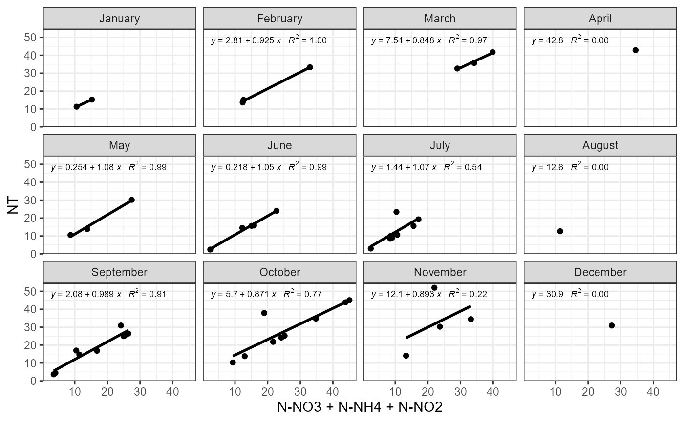
##
## $fraction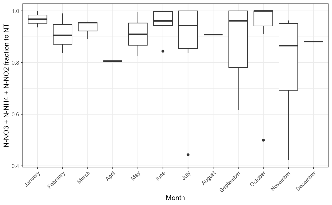
Example of function use with nitrogen.
plot_fractions(cal_data$data, station = c("4"), c("PT"), c("P-PO4"))## $regression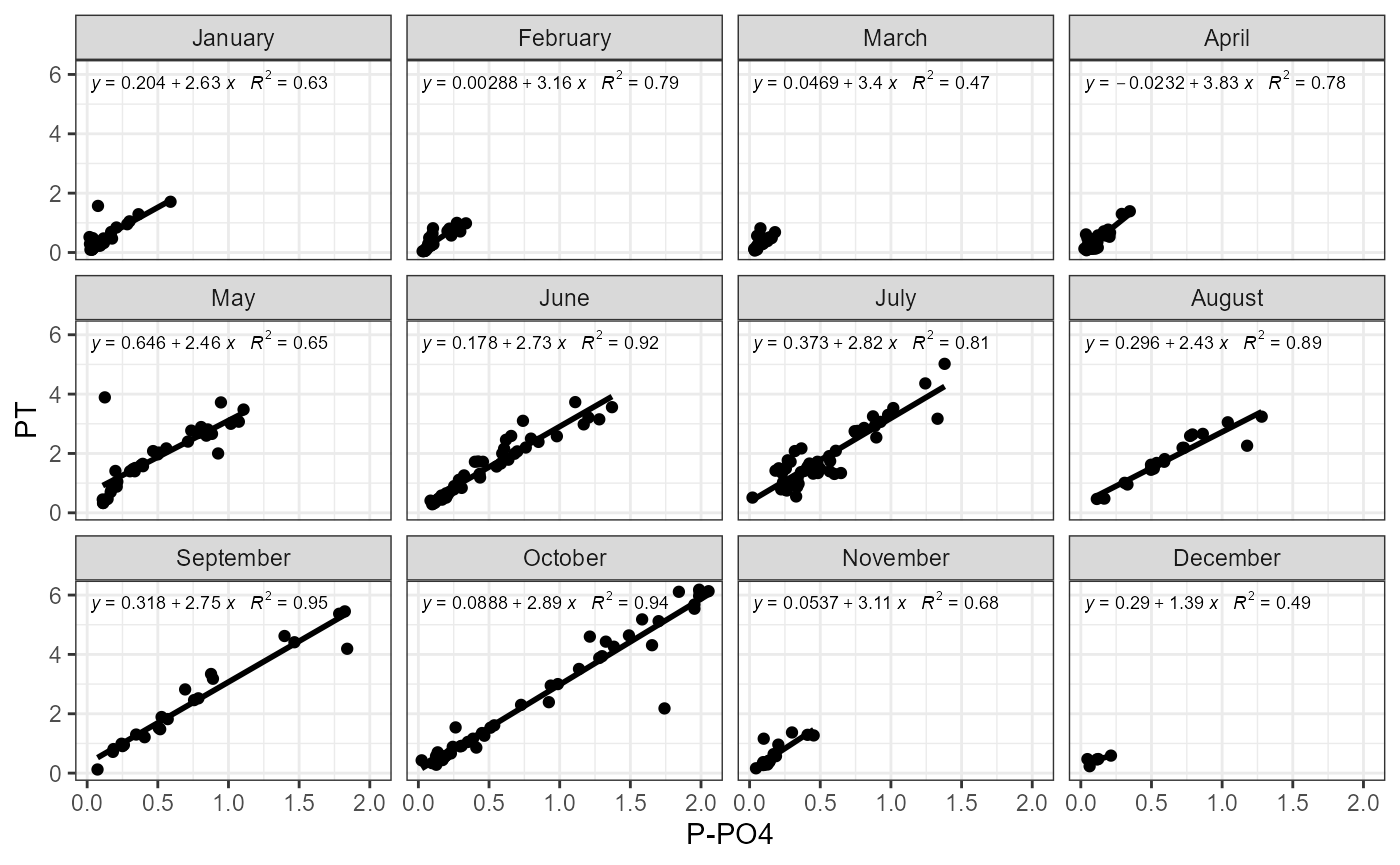
##
## $fraction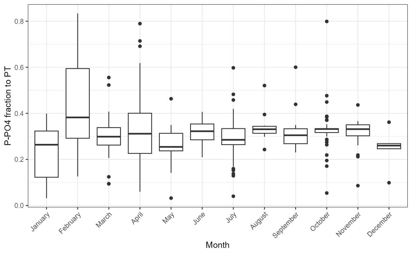
Maps
The last function in the package for plotting calibration data is plot_map. This function allows to plot catchment boundary, all monitoring stations and monitoring data within those station (press on monitoring station). This allow examination of spatial and temporal dimensions of existing data at the same time.
library(sf)
##Loading and converting coordinate system of GIS data. EPSG 4326 coordinate system should be used to get right plot.
reach_path <- system.file("extdata", "GIS/reaches.shp", package = "svatools")
basin_path <- system.file("extdata", "GIS/basin.shp", package = "svatools")
reach <- st_transform(st_read(reach_path, quiet = TRUE), 4326)
basin <-st_transform(st_read(basin_path, quiet = TRUE), 4326)
plot_map(cal_data$data, cal_data$stations, reach, basin)