The first step analyzes the model simulated weather inputs and water balance components. A comparison to literature values and observation data allows the user to verify if the weather input data are interpreted correctly and water balance results are plausible.
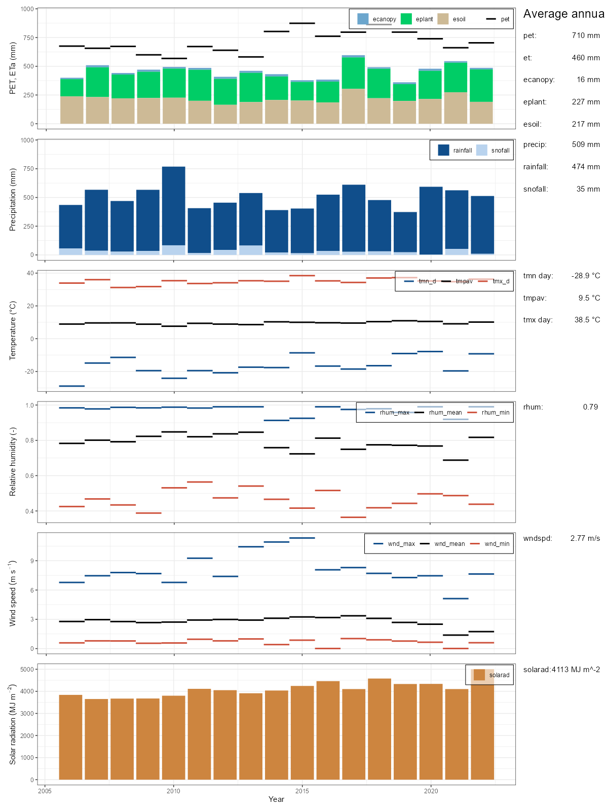
1. Analysis of simulated annual climate variables
The plot below gives an overview of the annual simulated basin average weather inputs. The simulated values should be in plausible ranges and must be comparable to literature values, before continuing with further model verification steps. The plot panels for relative humidity and wind speed will show all 0 values if a SWAT+ model revision lower than 60.5.5 was used in the simulation. A verification of the simulated relative humidity and wind speed cannot be done with this plot then. Please consider the points in the following checklist to verify the simulated weather data:
PET and ET
- Is the average annual PET plausible compared to regional PET?
- Is the variability of PET plausible?
>> The simulation of PET is influenced by weather inputs such as temperature, relative humidity, wind speed, and solar radiation. Simulated values which significantly differ to region specific literature values can indicate issues with other weather inputs (see also other plot panels).
>> Adjustments of PET can be achieved by small (!) changes in
the parameter pet_pmpt (which may be considered in the
water balance soft calibration).
- Is the average annual ET plausible compared to regional ET (if available)?
- Are the proportions between
eplant,esoil, andecanopyreasonable. In vegetated areaseplantshould be the dominant part ofet.
>> Low overall et can indicate issues in the
simulation of plant growth.
>> Low eplant compared to esoil can
indicate issues in the simulation of plant growth.
Precipitation and snow fall
- Are the annual precipitation sums in a plausible range?
- Is the fraction of snowfall compared to the precipitation sum plausible?
>> Large differences between simulated and observed precipitation can indicate issues in the precipitation input data.
>> If snowfall strongly differs from expected values this can
indicate issues with the temperature input data, or model parameters
such as snofall_tmp (snowfall temperature).
Temperature
- Are the daily minimum and maximum temperatures in plausible ranges?
- Are the annual mean temperature values and the average annual mean temperature comparable to region specific temperature statistics?
2. Seasonal dynamics of the precipitation and snow processes
This is an optional check for catchments where snowfall and snowmelt play a role. The upper plot panel shows the monthly average sums of precipitation separated into rainfall and snowfall. The plot should help to verify if start and end month seem plausible for snowfall to occur and if the fractions of snowfall compared to the total precipitation seem plausible.
The second plot panel shows the runoff that is generated by snowmelt. This plot should help to verify the snomelt dominated runoff in spring.
If the weather inputs were verified in the section above and no major
issues are present in the weather inputs, any visible issues in this
verification step can indicate problematic parametrizations of the SWAT+
snow parameters such as snofall_tmp (snowfall temperature)
and snomelt_tmp (snowmelt temperature).
plot_monthly_snow(sim_nostress)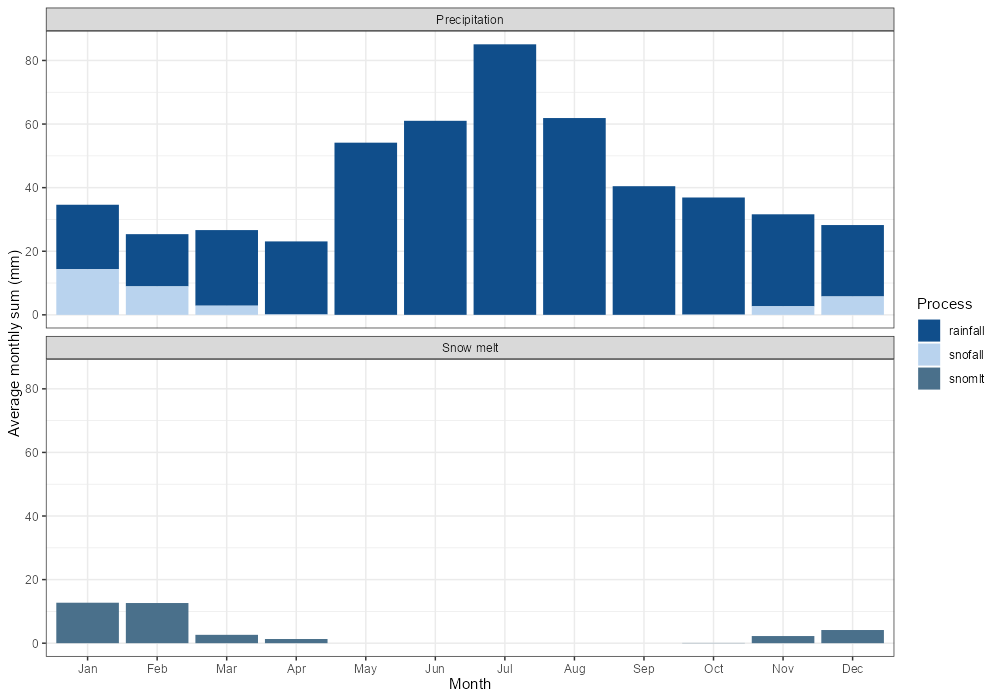
3. Overall simulated water balance
The plot below gives an overview of the overall simulated water balance. The water balance will be addressed in the soft calibration. It can be worth to have a quick look on the basin water balance components the verify if their shares of the overall water cycle are plausible and how the water yield ratio (wyld / precip) and the base flow ratio (base / wyld) already compare to the characteristics of the observed runoff. Some of the water balance components are also part of the weather inputs analysis. But this plots puts all components of the water cycle into perspective. You may have a look at the following aspects of the water balance:
Is the
wyldalready in a plausible range or is it excessive or 0?Are all components of
wyld(surface, lateral, and aquifer flow) active or is one of the components 0?Is the soil water storage in a plausible range (e.g. values much larger than 0 mm (e.g. ~ 100 mm) and lower than 600 mm)?
Does water percolate to the aquifer. Otherwise groundwater flow cannot occur?
If irrigation is implemented, is the value of
irr> 0?
Two versions of plot_waterbalance function are
available. The simplified version might be good to get overview, but the
detailed version is more important to quality assurance. Below are two
plots.
plot_waterbalance(sim_nostress, simplified = TRUE)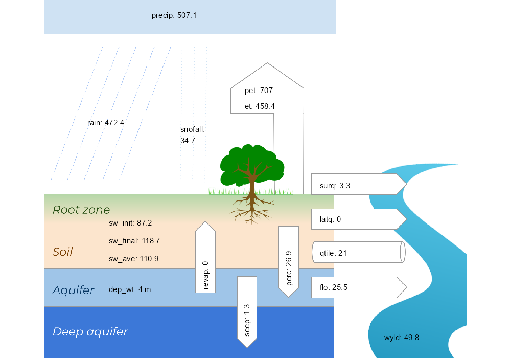
plot_waterbalance(sim_nostress)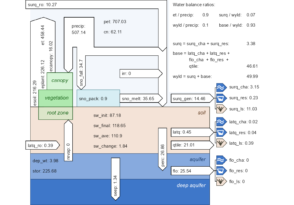
4. Analysis of simulated water balance at the HRU level
check_hru_waterbalance performs some checks for the
simulated water balance components to identify potential issues. Most of
the rules that were used in the check functions are adopted from
SWATCheck (SWATCheck however performs the analyses at a basin and land
use level). The returned table shows all HRUs for which at least one of
the checks identified a potential issue. The checks should help to
identify HRUs and land uses which should be further investigated
(e.g. with daily time series plots of the variables using the functions
plot_hru_pw_day or plot_hru_var). In the
example below checks were run for ET (et), soil water
(sw), and the curve number (cn). Some land
uses may always flag issues for some of the checks. So in the example
below they were ignored in the checks.
ignore_lum = c('^u', '^wet') means that all landuses which
begin with the letter ‘u’ (in this case urban land uses) and all wetland
land uses (begin with ‘wet’) were ignored.
hru_wb_check <- check_hru_waterbalance(sim_nostress,
                                       check = c('et', 'sw', 'cn'),
                                       ignore_lum = c('^u', '^wet'))
rmarkdown::paged_table(hru_wb_check)
To continue the analysis, please proceed to step 2.