Validation

This page corresponds to the 05_validate.R script in the hard calibration workflow. It provides a simple example of model validation. The validation workflow is similar to the calibration workflow, with the main difference being that only selected parameter sets are used for the model runs.

1. Load packages and settings

In the first step, the script loads the required packages, then it defines the model path and validation period, sets the simulation start and end dates, configures parallel processing, and specifies file names and paths for saving results. It selects the parameter sets for the validation runs.

# Load required R packages (if not yet done)-------------------------------
library(SWATrunR)
library(SWATtunR)
library(hydroGOF)
library(tidyverse)

# Path to the SWAT+ project folder.
model_path <- ''

## Define the period for which validate the calibrated model
period_valid <- c('yyyy-mm-dd', 'yyyy-mm-dd')

# Start date of the simulation for the validation period.
# This should be at least 2 years before 'start_date_print' and the start of the
# validation period to ensure the model reaches a steady state.
start_date <- 'yyyy-mm-dd'
# End date of simulation of validation period
end_date <- period_valid[2]
# Start date for printing of validation simulation outputs
start_date_print <- period_valid[1]

# Number of cores used for parallel simulation runs
n_cores <- NULL

# Name of the folder where simulation results will be saved incrementally.
# To continue writing to existing saved runs, replace by the name of the
# existing save_file.
save_file_name <- paste0(format(Sys.time(), '%Y%m%d%H%M'), '_sim_val')

# Path where the simulation results are saved.
# Default the simulations are saved in the calibration project
# in the sub-folder /simulation
save_path <- './simulation'

# E.g. path to discharge observations
flow_path <- './observation/.csv'

## The main step in valitadion is to run only selected parameter sets
parameter_set_valid <- parameter_set[run_ids, ]

2. Perform simulation runs and load results

In this step, the script performs the simulation runs using the validated parameter and loads the simulation results, observation data for further analysis.

# Perform simulation runs
run_swatplus(project_path     = model_path,
             output           = outputs,
             parameter        = parameter_set_valid,
             start_date       = start_date,
             end_date         = end_date,
             start_date_print = start_date_print,
             n_thread         = n_cores,
             save_path        = save_path,
             save_file        = save_file_name,
             return_output    = FALSE,
             split_units      = FALSE, # better set TRUE for large number of units
             time_out         = 3600 # seconds, change if run-time differs
)

# Parameter definition ----------------------------------------------------
# Paths to simulation and observation data
# E.g. load the simulations with the last time stamp, if default
# save_file names in simulation runs is used.
sims <- list.files('./simulation/', pattern = '[0-9]{12}_sim_val')
sim_path <- paste0('./simulation/', sims[length(sims)])

# Load and prepare simulation results -------------------------------------
sim <- load_swat_run(sim_path)

# E.g. discharge observations
flow_obs <- read_csv(flow_path) %>%
  filter_period(., period_valid)

flow_sim <- filter_period(sim$simulation$flo_day, period_valid)

3. Analyze results

In this step, the script evaluates the model performance. It first calculates the flow duration curves (FDCs) for simulated and observed discharges. Then, it computes goodness-of-fit (GOF) metrics such as NSE, KGE, PBIAS, and MAE for discharge, and evaluates RSR values across different FDC segments. The results are combined into a single table, from which selected GOF values are extracted. Finally, it summarizes the mean performance metrics across all runs, with options for further analysis or plotting provided in a separate script.

# E.g. if FDC segments should be evaluated, calculate the
# FDC for the simulated discharges
flow_fdc_sim <- calc_fdc(flow_sim)
# E.g. if FDC segments should be evaluated, calculate the
# FDC for the simulated discharges
flow_fdc_obs <- calc_fdc(flow_obs)

# Calculate goodness-of-fit values ----------------------------------------
# E.g. to calculate typical indices such as NSE, KGE, pbias, etc. for discharge
gof_flow <- calc_gof(sim = flow_sim, obs = flow_obs,
                     funs = list(nse_q = NSE, kge_q = KGE, pb_q = pbias,
                                 mae_q = mae))

# Calculate RSR for different discharge FDC sections (as proposed in
# Pfannerstill et al., 2014 (https://doi.org/10.1016/j.jhydrol.2013.12.044))
gof_fdc <- calc_fdc_rsr(fdc_sim = flow_fdc_sim, fdc_obs = flow_fdc_obs,
                        quantile_splits = c(5, 20, 70, 95))

# E.g. if all calculated GOF tables should be joined to one table
gof_all <- list(gof_flow, gof_fdc) %>%
  reduce(., left_join, by = 'run')

# Select the GOF values of interest
gof_sel <- select(gof_all, run, nse_q, pb_q, p_0_5, p_20_70, p_70_95)

# Print the mean GOF values for all runs
gof_sel[names(gof_sel)[names(gof_sel) != "run"]] %>% summarise_all(mean)

# For plotting options or extension to different variables, etc., see the the
# 04_analyze_results.R script.

For plotting options, please refer to this page for guidance on visualizing the results, as well as the 04_analyze_results.R script.

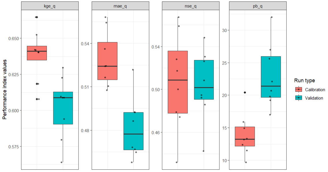
If you are satisfied with the validation results, it is advisable to check for any underlying issues in the model setup before proceeding to scenario modeling. This can be done using the SWAT+ model setup verification workflow described here, which helps identify potential issues and can save considerable time in later stages of model use. The quality assurance step is particularly important if the model will be applied to scenario analysis for decision-making.

Validation of model performance using selected parameter sets

1. Load packages and settings

2. Perform simulation runs and load results

3. Analyze results