Calibration data

Introduction

Calibration and validation data are required for model input. However, these data are necessary for assessing model performance. As it is usually collected and prepared during data gathering stage, SWATprepR includes functions to quickly load into R, assess, plot and clean monitoring data. For more information about required data and calibration/validation step please see chapter 6 in SWAT+ modeling protocol.

Loading

Data, which are prepared according to given template (‘calibration_data.xlsx’), can be loaded directly with package function load_template. Function loads data into a list with two dataframes. First one is for station information (location, name, ID). Second - for values from those monitoring stations with IDs to relate to station, variable names, dates and values. Function needs only path to a template and EPSG code (if different from 4326) for setting correctly point coordinates.

library(SWATprepR)
library(sf)
temp_path <- system.file("extdata", "calibration_data.xlsx", package = "SWATprepR")
cal_data <- load_template(temp_path, epsg_code = 4326)

## [1] "Loading data from template."
## [1] "Loading of data is finished."

Example of loaded data structure presented below.

str(cal_data)

## List of 2
##  $ stations: sf [24 × 6] (S3: sf/tbl_df/tbl/data.frame)
##   ..$ ID         : chr [1:24] "5" "8" "4" "2" ...
##   ..$ Name       : chr [1:24] "Zgłowiączka-Strózewo-Parcele" "DopZStarRadziejewa - Witowo" "Zgłąwiączka-ponizej. Osiecin,Samszyce" "Zgłowiączka-pow.Osiecin. Piołunowo" ...
##   ..$ Description: chr [1:24] "powyżej jez. Głuszyńskiego (60 km)" "Kolonia Witowo" "Samszyce - poniżej Osięcin (67,8 km)" "powyżej Osięcin (75,2 km)" ...
##   ..$ geometry   :sfc_POINT of length 24; first list element:  'XY' num [1:2] 18.7 52.6
##   ..$ Long       : num [1:24] 18.7 18.7 18.7 18.7 18.7 ...
##   ..$ Lat        : num [1:24] 52.6 52.6 52.6 52.6 52.6 ...
##   ..- attr(*, "sf_column")= chr "geometry"
##   ..- attr(*, "agr")= Factor w/ 3 levels "constant","aggregate",..: NA NA NA NA NA
##   .. ..- attr(*, "names")= chr [1:5] "ID" "Name" "Description" "Long" ...
##  $ data    : tibble [33,261 × 5] (S3: tbl_df/tbl/data.frame)
##   ..$ Station  : chr [1:33261] "1" "1" "1" "1" ...
##   ..$ DATE     : POSIXct[1:33261], format: "2008-03-11" "2008-03-25" ...
##   ..$ Variables: chr [1:33261] "N-NH4" "N-NH4" "N-NH4" "N-NH4" ...
##   ..$ Values   : num [1:33261] 0.05 0.05 0.05 0.05 0.05 0.05 0.83 0.25 0.51 1.89 ...
##   ..$ Source   : chr [1:33261] "grab sample" "grab sample" "grab sample" "grab sample" ...

Plotting

The first thing after loading data is plotting it to assess its quality.

Timeseries

There are several ways package could be used to plot loaded calibration data. Data for multiple stations could be interactively plotted using plot_cal_data function. This function should be used on several stations with relatively few data points to screen for data coverage and potential problems.

plot_cal_data(cal_data$data, c("3","10"))

For data rich monitoring station plot_cal_data function should be used only with single station selected. Such plotting allows better visualization.

plot_cal_data(cal_data$data, c("4"))

Monthly summary

Sometimes for the evaluation of data quality monthly plots can be useful. Such plots allow to see if monitoring results corresponds to other data sources and processes, which should be taking place in a monitored catchment. plot_monthly function can be used to interactively plot monthly aggregates.

plot_monthly(cal_data$data, station = "4")

Fractions

Possible problems could be observed plotting how mineral and total parts of nutrients compares between months. plot_fractions could be used for nitrogen and phosphorus. Function provides monthly regression and monthly fraction figures.

Example of function use with nitrogen.

plot_fractions(cal_data$data, station = c("4"), c("NT"), c("N-NO3", "N-NH4", "N-NO2"))

## $regression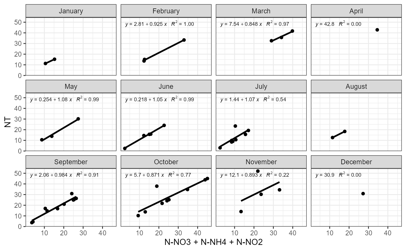

## 
## $fraction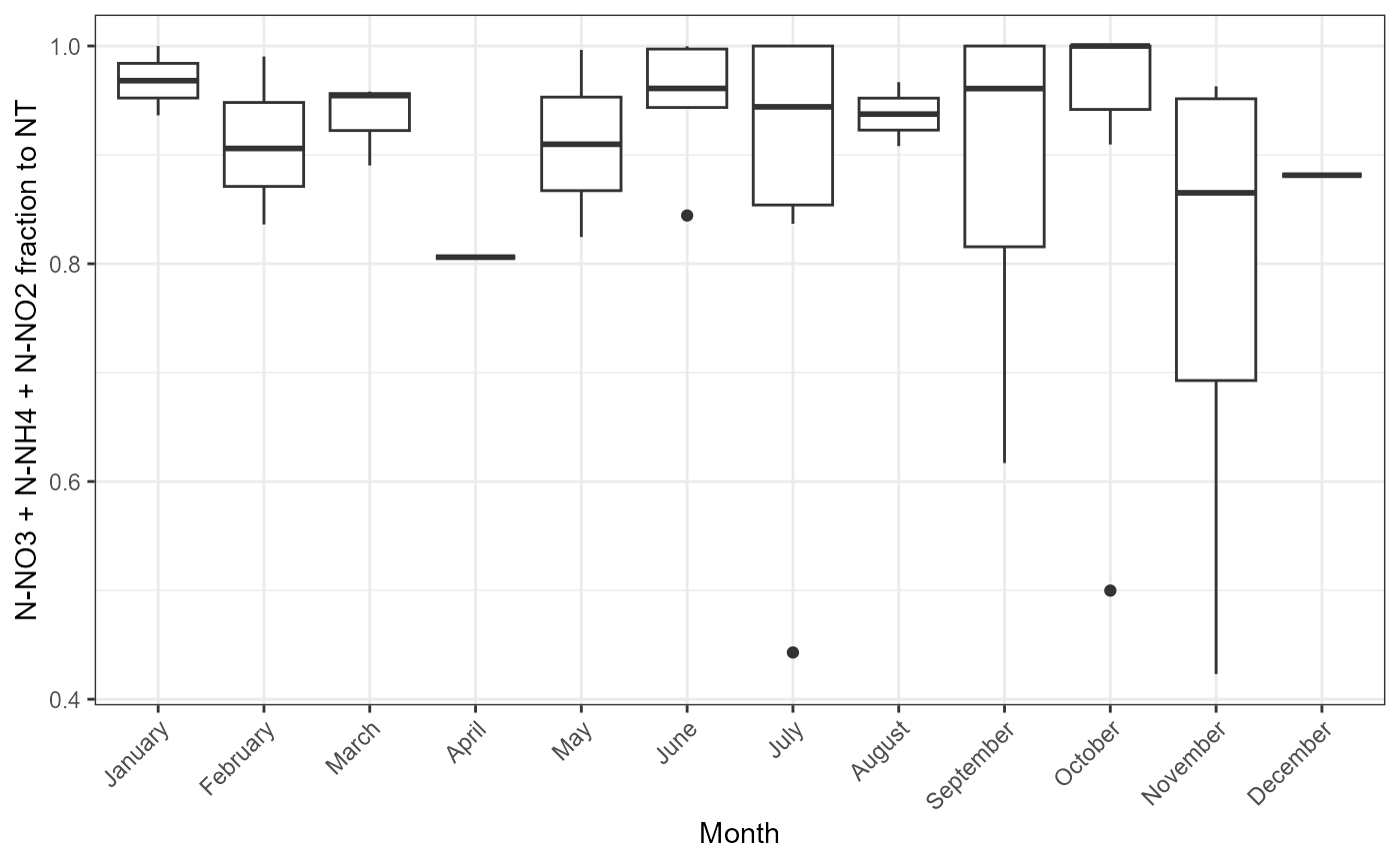

Example of function use with phosphorus.

plot_fractions(cal_data$data, station = c("4"), c("PT"), c("P-PO4"))

## $regression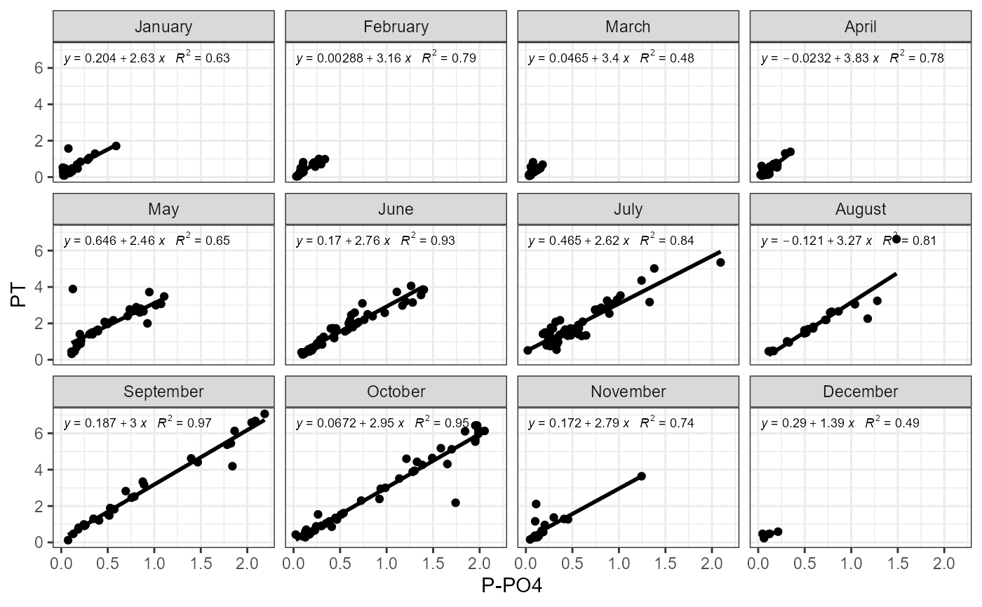

## 
## $fraction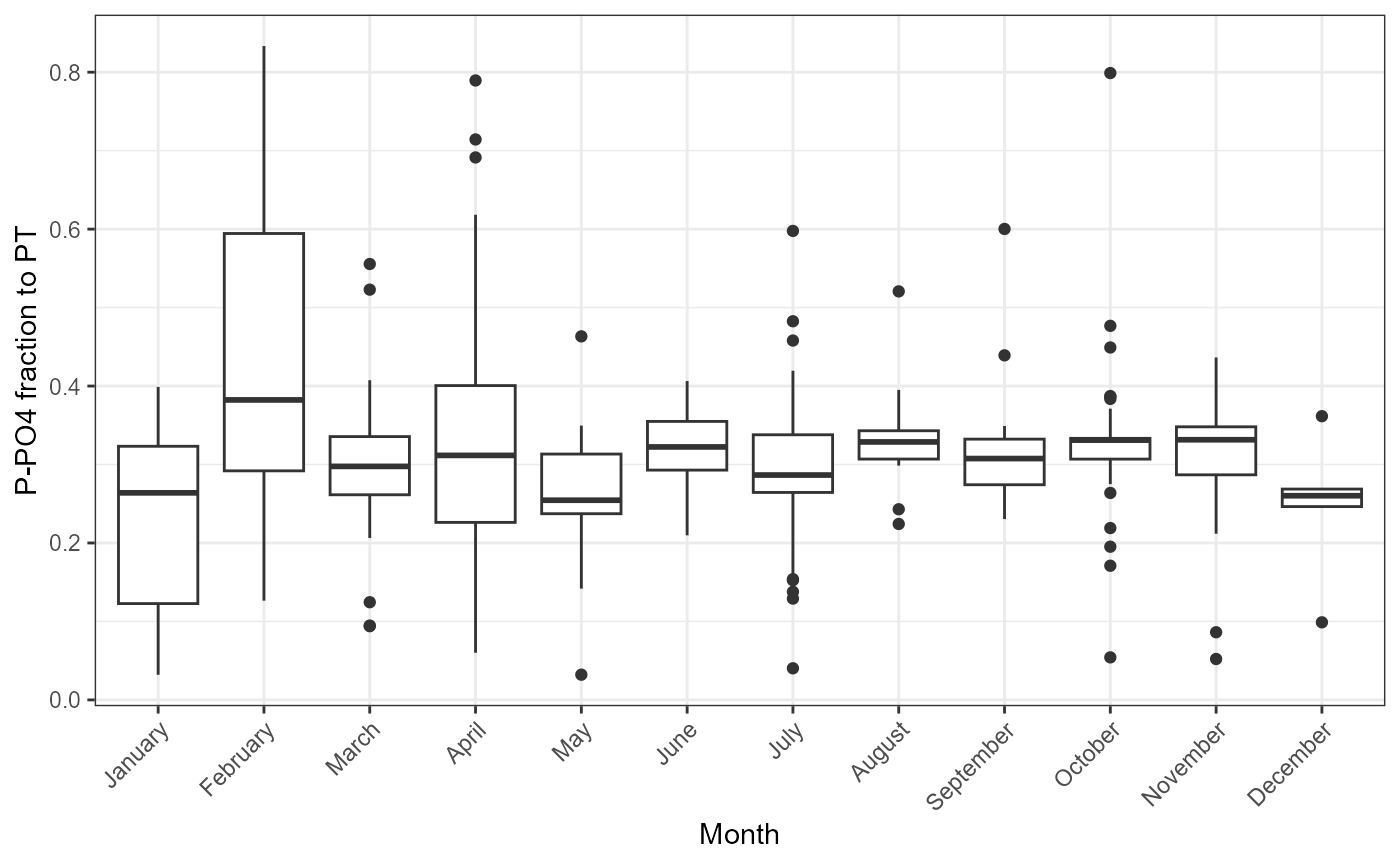

Maps

The last function in the package for plotting calibration data is plot_map. This function allows to plot catchment boundary, all monitoring stations and monitoring data within those station (to see data press on monitoring station). This allow examination of spatial and temporal dimensions of existing data at the same time.

library(sf) 
##Loading and converting coordinate system of GIS data. EPSG 4326 coordinate system should be used to get right plot. 
reach_path <- system.file("extdata", "GIS/reaches.shp", package = "SWATprepR")
basin_path <- system.file("extdata", "GIS/basin.shp", package = "SWATprepR")
reach <- st_transform(st_read(reach_path, quiet = TRUE), 4326)
basin <-st_transform(st_read(basin_path, quiet = TRUE), 4326)
plot_map(cal_data$data, cal_data$stations, reach, basin)

Cleaning

Two functions could be applied for data cleaning. First is clean_wq function, which could be applied for fixing most common water data issues as fixing data formats, units (e.g. NO₃, to N-NO₃), instead of LOD/LOQ values using LOD or LOQ divided by 2, replacing zeros from water quality variables with minimum value (multiplied by selected coefficient) for variable.

##Zeros is replaced with min(Value)/2
cal_data$data <- clean_wq(cal_data$data)

Second function clean_outliers allows removal of suspicious values defined as being outside selected range (mean - standard deviation; mean + standard deviation). This function provides list of two dataframes. One is for data to be removed, the other - for data to be left.

lst <- clean_outliers(cal_data$data)

Example of data to be removed.

##Looking at data to be removed
print(head(lst$dropped))

## # A tibble: 6 × 5
##   Station DATE                Variables Values Source     
##   <chr>   <dttm>              <chr>      <dbl> <chr>      
## 1 10      2012-11-26 00:00:00 N-NH4      22.1  grab sample
## 2 10      2012-12-11 00:00:00 N-NH4      16.8  grab sample
## 3 10      2016-02-04 00:00:00 N-NH4       6    grab sample
## 4 10      2016-03-07 00:00:00 N-NH4       4.67 grab sample
## 5 10      2016-04-04 00:00:00 N-NH4      11.1  grab sample
## 6 10      2016-07-15 00:00:00 N-NH4      14.9  grab sample

To remove outliers from data following line could be used.

##Updating data
cal_data$data <- lst$newdf